Introduction
Transformers are the largest ML workloads of today.
Probabilistic co-design is central to Extropic's mission of creating more energy-efficient computational systems. We have already -- we've spent years advancing hardware-algorithm co-design for thermodynamic and probabilistic computers.[1][2]
However, the algorithms of today are almost entirely dominated by a singular Transformer[6] architecture. Perceived demandDemand for this architecture has led to one of the largest industrial buildouts in recent history, which is both extremely costly[7] and extremely energy demanding.[8][9]
To address these growing issues, we investigate how our upcoming probabilistic subthresholdsub-threshold CMOS chip, Z1, can potentially be used to increasebe used to improve the energy efficiency of transformer-like models. Z1 was designed as a probabilistic graphical model sampler, and not with neural networks, much less transformers, in mind. Nevertheless, we can deriveWe derive inspiration from the Boltzmann-machine lineage of neural computation[11] to run sparse neural layers on Z1. We use this idea to build Z1T, combining it with the neighboring FPGA on Z1. In a hybrid mode, this companion processor could instead be a GPU or another accelerator, though our concrete estimates use the FPGA.Pairing Z1 with an FPGA on the same board gives us Z1 Transformer (Z1T).
Note: The companion processor could in principle be a GPU or another accelerator, but all estimates here assume the FPGA.
Here we report our preliminary investigation into this direction for heterogeneous decode disaggregation. We outline below the components of the transformer-like architecture we constructed, how we can break down layers and divvy up the computations between Z1 chips and FPGAs, and how much energy this decoding pass requires relative to an H100 GPU.
This is an initial study in sparse neural-network and hardware co-design. While the design of Z1 predates these ideas, we are using them to inform future chips that can improve the performance of Z1T-style models.
Scaling
Empirical scaling sweeps for sparse models
The modern era of deep learning is defined by somewhat predictable scaling[12][13] given the training dataset size, compute, and loss. Sparse hardware introduces another variable into this equation: connectivity. This is important for this work, asmatters as Z1 has fixed connectivity embedded in the silicon. Gaining insight into the scaling propertiesUnderstanding scaling behavior is essential for co-design, as informing future chips requires predicting what will scale. There are a number of open questions, such as how does loss change for fixed compute and data but changing sparsity? Does sparse training scale generally the same (given that for the same number of FLOPs, you have deeper/wider models)? What are the highest value levers for Z2?:
- How does loss change with sparsity and connectivity at fixed compute and data?
- How do sparse scaling trends compare to dense model scaling?
- What are the design levers matter most for our next chip, Z2?
We investigate these questions in two directions.: First, we build a gated convolutional attention (GCA)[14] architecture whose sparse tanh-linear projections map naturally to Z1. Second, we vary a shared connectivity parameter in a standard decoder transformer to study sparse projections and shortened attention context away from the Z1-specific operations.
A transformer built for Z1
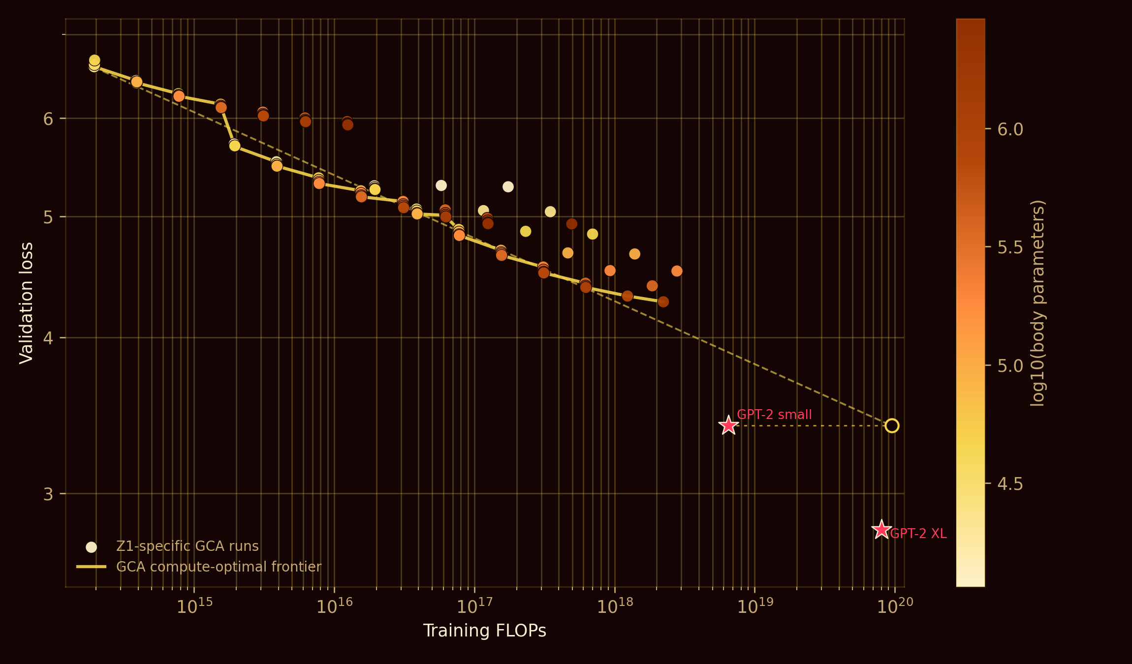
We sweep the Z1-matched architecture. Technical details appear in the architecture section below. With 4-bit quantization and four incoming edges per output node, we can run models that respect the Z1 pattern. We then use the FPGA for non-Z1-compatible operations. We consider this an optimized architecture for utilizing Z1. Below, we plot the loss scaling given FLOPs and parameters on the OpenWebText dataset with the GPT-2 byte-pair encoding (BPE) tokenizer. We sweep model size for an architecture matched to Z1's constraints: 4-bit weights and four incoming edges per output node (see the architecture section for details). We then use the FPGA for non-Z1-compatible operations. This split is our best-performing configuration for Z1. Below we plot loss against FLOPs and parameter count, trained on OpenWebText with the GPT-2 byte-pair encoding (BPE) tokenizer.
General sparsity considerations
We focus first on the general effect of sparsity in transformer models. We want to know how important sparsity is when added as an axis in the standard scaling law formula to help inform future decisions around connectivity. This model is a standard GPT-2 style decoder, with dot-product masked self attention, RMS normalization[16], and GELU[17] based feed forward blocks. We then train it on byte-tokenized OpenWebText.
In these experiments, we have a single additional knob, the: connectivity c. This controls two parts of the models, both the matrix multiplications (e.g. the WQ, WK, WV projections, and the feed forward blocks), and the attention scores (via windowed attention). For c = N, each output node of the network is connected to N input nodes (e.g. the row of W in W @ x has N non-zero values), the attention scores are also windowed to the last N values.
Importantly, this is a fixed connectivity pattern, not a percentage sparsity. This differs from the usual sparse neural models which operate under fixed, e.g. 95%, sparsity considerations. As width increases, our percentage sparsity asymptotically becomes 100%. This is due to the fact that we have to fix the connectivity in silicon and thus have this unique factor. In our experiments, this percentage varies from 5% to 99.8%.
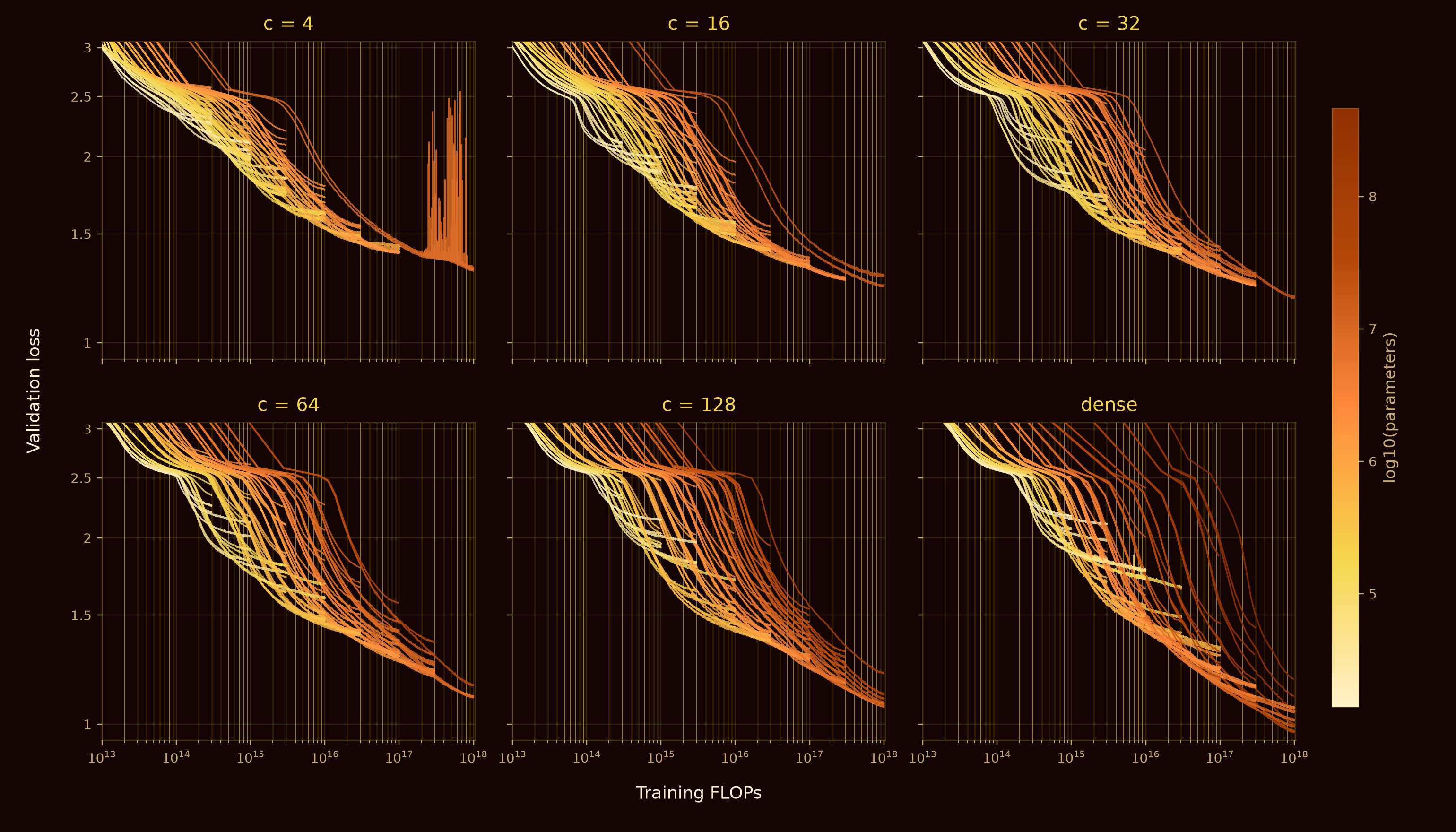
We benchmark c ∈ {4, 16, 32, 64, 128} on sequence length 256, in addition to a fully dense baseline, from 3×10¹⁴ FLOPs to 1018.
First we plot the loss vs. the training FLOPs for a variety of sparsities and parameters. All parameters in these plots include both body parameters and the final (always dense) matrix.
We then investigate the iso-FLOP curves. Importantly, to achieve the same number of parameters with lower connectivity, the models must be (sometimes substantially) deeper and wider than the dense model.
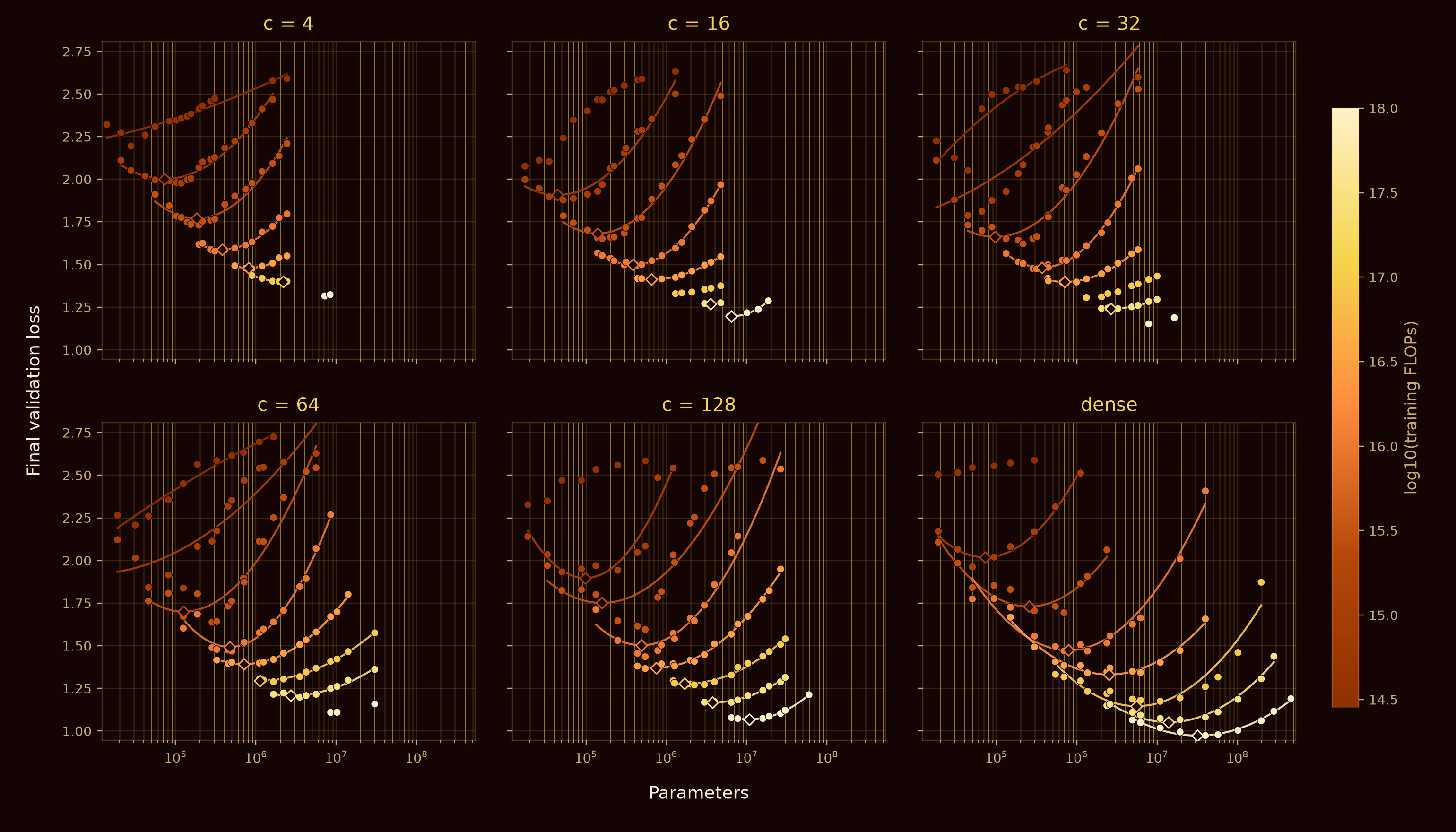
While dense models in these early results seem more efficient per FLOP, sparse Z1 FLOPs are massively more energy-efficient than GPU-based computation, thus sparse models running on Z1 can still be orders of magnitude more power efficient at the same level of model performance, as we will see below. These early results suggest dense models are more efficient per FLOP -- however, a sparse FLOP on Z1 costs far less energy than the equivalent operation on a GPU, so a sparse model on Z1 can still reach the same performance at a fraction of the power, as we show below.
The hardware
Z1: A naturally sparse chip.
Our chip, Z1, is built as a graphical model of probabilistic bits (pbits). These are binary stochastic CMOS circuits whose probability is controlled by a bias induced by neighboring pbits.[19] The chip is organized as an Ising model[3] and updates the states via Gibbs sampling[20] at a 50 MHz internal update clock. Each pbit draws a new value conditioned on its neighbors, executing a chromatic Gibbs sampling algorithm in-memory.
This neighbor graph is fixed in silicon, of degree 16, for a total of 269,568 pbits and 2,135,904 edges on a single chip. On Z1, computation exists only where there is a physical coupling for it: a program maps directly onto the chip only if its interaction graph is a subgraph of the fixed coupling graph. This is unlike GPUs which achieve all-to-all "connectivity" between cores by having a cache memory hierarchy which all units have access to. Modern GPUs are optimized for large, regular, dense matrix multiplications.[10] Sparse operations on a GPU can create irregular memory access patterns, while simultaneously not providing any speedups proportional to their sparsity levels.[21]
Z1T does not run a dense layer unchanged on the probabilistic substrate. Instead, it refactors the layer around the hardware's fixed sparse connectivity. These estimates assume enough Z1 chips running in parallel to place all samples. For a single unit of Z1, the energy of the visible node and its 16 neighbors is Z1T doesn't drop a dense layer onto the chip as is -- instead, it rewrites the layer to compile onto the chip's fixed sparse topology. The numbers below assume you have enough Z1 chips running side by side to place all samples. For one Z1 unit, the energy of a visible node and its 16 neighbors is:
Hardware encoding
Embedding operations on a sparse probabilistic chip
Encoding continuous numbers into pbits
Neural-network activations and weights are typically floating-point values, while Z1 operates on pbits (which can also be represented as spins over {−1, 1}). To operate on continuous values with Z1, we need a way to map continuous numbers to pbit representations. Fundamentally this involves quantizing the continuous value into some number of pbits.
While there are a variety of schemes that could be considered, for example:
We refer to this as the dy4p quantization of x: dyadic, because every scale is a power of two, with 4 bits of precision. This dy4p could be seen as the spin analogue of a 4-pbit probabilistic integer (p-Int) encoding, pInt4.
One key building block of our components for Z1T is the tanh-linear unit, constructed from averaging one probabilistic cell. For one tanh-linear element of Z1, the energy of a visible node and its 16 neighbors is:
Conditioning on the hidden nodes, the visible spin is a Bernoulli distribution over {−1, 1} which when averaged becomes a tanh of the local field.
This tanh-linear unit can be applied in parallel for each output node.
A weighted activation can therefore be written as the expectation of a pbit with:
This also extends to vectors. For an input x ∈ ℝD and spins s ∈ {−1,+1}D×4 with 4 spins per value, the weight matrix can be directly encoded into the interactions over the flattened spin vector via:
The hardware naturally samples from a distribution whose expectation is a sparse matrix-vector product fused with a tanh. We can leverage these units to do tanh-linear operations that are similar to a component of a neural network. In this work we assume that one has sufficient Z1 chips running side by side to place all sampled tanh-linears in a model-parallel fashion. While these encodings are necessary for practical Z1 execution, the results of Figure 1 do not include quantization of the activations.

Model architecture
Z1T keeps the transformer outline but modifies its primitives.
A traditional Transformer block[6] typically is constructed from a Self Attention block, a RMSNorm and a FeedForward Network. These primitives rely on dense matrix operations, and thus are typically deployed on GPUs. In this investigation, we try to adapt these primitives to the sparse tanh-linear layers we can run on our Z1 chip.
The RMSNorm layer is implemented as:
Empirically it has been shown that each component of RMSNorm resembles a tanh activation, and can be replaced with a scaled Dynamic Tanh (DyT).[22] We can therefore substitute RMSNorm components with the DyT:
This is naturally implementable on Z1 by fusing the shift and scale with subsequent layers.
Classic softmax-based attention is computed using dense queries, keys and values matrices. Given an input sequence X ∈ ℝT×D and projection matrices WQ, WK, WV ∈ ℝD×D, we compute Q = XWQ, K = XWK, V = XWV. Self attention is then
This requires O(T2D) sequence work and dense matrix multiplication to encode the query-key scores. We instead adapt a gated convolutional attention architecture to sparse hardware.[14] Given our token stream X, we instead use 4-sparse projection matrices to compute the gates Q, K, V. At a token in position t, head i:
We can offload certain arithmetic and transcendental functions to an XPU. Our systems use an FPGA as a coprocessor, which allows for flexible operations and energy efficiency.
A simple feed-forward network can be mapped to our hardware by composing tanh sampling programs across the chip fabric. An MLP layer is given by
For a sparse W we can compile[3] this to hardware by laying out dout many tanh-linear units on Z1 and stream the samples between the cores.
Mechanism
Watch one position move through gated convolutional attention
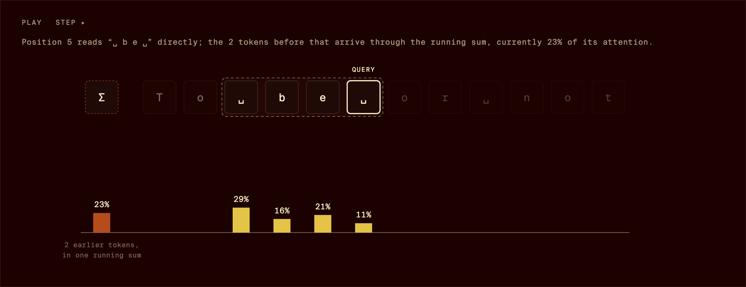
Fig. 5 Visualization of gated convolutional attention and the sequence of operations being applied on a token going through the mechanism.
Token trace
Follow one token across the FPGA and Z1.
Here we follow the journey of a token as it crosses between being processed on the FPGA and Z1.
The FPGA adds each block's input back around the attention and MLP transforms. It also runs the vocabulary readout that produces the logits, and Z1 samples the next token.
In this investigation, we've used an FPGA to get concrete estimates quickly. However, the dense vocabulary matmul and much of the remaining digital work could run on other accelerators, such as GPUs or dedicated accelerators from Cerebras, Etched, etc.
These early results suggest dense models are more efficient per FLOP. However, a sparse FLOP on Z1 costs far less energy than the equivalent operation on a GPU. Moreover, a sparse model can reach the same performance at a fraction of the power, as we show below.
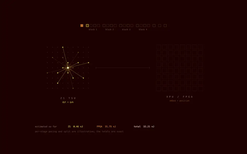
Energy cost model
The modeled block uses up to 139× less energy per token than an H100.
Energy efficiency gains
Note that the following projections are based on theoretical chip energy consumption of Z1 based on our best estimates, which are anchored to reality from our experiments with similar pbits in X0. We exclude the dense logit final readout layer of computation in these estimates.
| H100 model FLOPs utilization | H100 energy / token | H100 / Z1T | H100 / Z1 layers |
|---|---|---|---|
| 10% | 40.9 µJ | ≈139× | ≈4,680× |
| 50% | 8.17 µJ | ≈28× | ≈935× |
| 100% | 4.09 µJ | ≈14× | ≈468× |
The first column is the model FLOPs utilization (MFU), the fraction of the theoretical peak H100 FLOPs reached by the measured throughput. In LLMs such as Llama 3, MFU is around 40%.[23] For very sparse models, which H100s are less optimized for, one often sees much lower MFU.
The H100 / Z1T is the energy ratio between inference (excluding the final dense logit computation) on the H100 and Z1 system. This system includes all previous computations done on both the Z1 fabric and the connected FPGA (but does not include data movement between the two). The last column compares the layers that just run on Z1 (i.e. sparse tanh layers).
Model details
- Z1 topology: 8 cores × 33,696 pbits = 269,568 pbits, 2,135,904 hardwired edges
- Z1 sampling energy: 1.3e-14 J per sample
- Card assumption: samples and channels are placed across parallel Z1 chips; the required chip count is not modeled
- FPGA estimate: 0.2 pJ/matrix-multiply op, 3.0 pJ/scalar op, 1.5 W assumed static power
- Model dimensions: L=4, D=512, T=1024, GCA H=4, kernel=4, sparse k=4
- H100 reference: 32-bit floating-point peak energy 0.177 pJ per floating-point operation, the same next-token step run densely, with no sparsity exploited, model FLOPs utilization varied above
The Z1T estimate is 294.52 nJ per token: 8.74 nJ for Z1 sampling and 285.78 nJ for the included FPGA work (including the final logit readout on a FPGA yields approximately 136.4 µJ per token).
Latency model
Throughput and latency
Assuming a single serial stream and no advanced pipelining methods, we estimate the throughput as follows.
Sampling Z1 accounts for ~16 µs of the larger estimate. Each sample is drawn in parallel on the fabric and averaged to get an estimation of the scalar tanh-linear output.
| Operating point | Latency / token | Tokens/sec |
|---|---|---|
| Z1T conservative | 58.8 µs | ≈17,000 |
| H100 eager PyTorch | 702 µs | ≈1,425 |
| H100 torch.compile | 102 µs | ≈9,764 |
For the H100 comparisons, we evaluated the speed with batch-1 sequential decoding of the model. In both the H100 and Z1 cases, we exclude the final vocab logit computation. Since this model is quite small relative to the scale of a H100, the kernel launch times play a non-negligible impact on speed (this model achieves 0.006% MFU). If we were to batch on the GPU, H100s would be substantially more efficient. As such, we advise using our Z1 + XPU setup for decode rather than prefill, which is better done on GPU for now.
Latency model details
- Steps: 25 sequential sampling layers, 8 FPGA-to-Z1 data writing steps, 5 Z1-to-FPGA data reading, FPGA computes all the rest such as pooling, positional-encoding, and residual work
- Estimated time breakdown: 38.0 µs for FPGA orchestration (38 serial ops × 1 µs), 16.0 µs Z1 sampling (25 × 32 samples at 50 MHz), 3.2 µs data reading, 1.3 µs data writing, 0.13 µs FPGA sample averaging, 0.16 µs FPGA pool/positional/residual = 58.8 µs total
- Z1 I/O: 25.6 Gbit/s data transfer speed
- These estimates are conservative as we do not count parallel samples. Note that parallelizing sampling would consume the same amount of energy, but parallelized samples would reduce the time to achieve certain desired precision due to the higher rate of sampling and reduction of empirical variance. Please refer to our section on probabilistic encoding of continuous numbers for the equivalence between samples and digital precision.
- H100 baseline: NVIDIA H100 80GB HBM3, torch 2.7.0, dense-equivalent model, D=512, L=4, 11.55M body parameters in fp16, measured 2026-08-12
Outlook
One small step for co-design. One giant leap for the densification of intelligence.
In this Z1T experiment, we evaluated how to put a transformer-like set of operations onto a joint probabilistic/FPGA fabric that was not originally designed for this set of operations. Even in this unoptimized regime, we found compelling energy efficiency gains at a time when energy consumption of ML models is a pressing issue.
Our energy estimates indicate that the FPGA consumes the vast majority (>95%) of the energy, which means that there are substantial improvements that could be made by a chip designed with transformer-like neural models like Z1T in mind. By shifting more of the operations onto an ultra-energy-efficient sub-threshold CMOS substrate, one could reap even larger energy savings, potentially reaching up to 1000× greater energy efficiency than GPUs. Removing the FPGA bottleneck would take this approach to that level, in line with the Z1-only layer gains reported above. We leave this for future algorithmic and hardware explorations. This work was only the beginning of our co-design journey coupling our chips to the world of transformers. Many more iterations to come.
References
References
- Lockwood, O., Béjanin, J., Bus, J., Chamberland, C., Huembeli, P., Schäfer, F., & Verdon, G. (2026). A Blueprint for Equilibrium-Based Differentiable Continuous-Variable Thermodynamic Computing. arXiv preprint arXiv:2607.16183. https://arxiv.org/abs/2607.16183↩
- Jelinčič, A., Lockwood, O., Garlapati, A., Schillinger, P., Chuang, I. L., Verdon, G., & McCourt, T. (2026). An Efficient Probabilistic Hardware Architecture for Diffusion-Like Models. npj Unconventional Computing, 3, Article 30. https://doi.org/10.1038/s44335-026-00075-3↩
- Extropic. (2026). From One to One Billion: Torx, Thermalizers, and Z1. https://extropic.ai/writing/from-one-to-one-billion↩
- Verdon, G., Tyrpak, L., Lockwood, O., Morton, S., Neagoe, A., Sugolov, A., MacCormack, I., & Amico, M. (2026). A Framework for Stochastic Differentiable Programming. arXiv preprint arXiv:2608.01612. https://arxiv.org/abs/2608.01612↩
- Amico, M., Jelinčič, A., Nancarrow, C. O., Tyrpak, L., Roberts, D., Morton, S., Sakthivadivel, D., Gopal, A., & Verdon, G. (2026). Thermalizing Stochastic Programs. arXiv preprint arXiv:2608.01615. https://arxiv.org/abs/2608.01615↩
- Vaswani, A., et al. (2017). Attention Is All You Need. Advances in Neural Information Processing Systems, 30. https://proceedings.neurips.cc/paper/2017/hash/3f5ee243547dee91fbd053c1c4a845aa-Abstract.html↩
- Whitwam, R. (2026, July 23). Google just had its first negative cash flow quarter due to massive AI spending. Ars Technica. https://arstechnica.com/google/2026/07/google-just-had-its-first-negative-cash-flow-quarter-ever-due-to-massive-ai-spending/↩
- International Energy Agency. (2025). Energy and AI. IEA. https://www.iea.org/reports/energy-and-ai/energy-supply-for-ai↩
- Congressional Research Service. (2026). Data centers and their energy consumption: Frequently asked questions (CRS Report No. R48646). https://www.congress.gov/crs-product/R48646↩
- Hooker, S. (2021). The Hardware Lottery. Communications of the ACM, 64(12), 58–65. https://doi.org/10.1145/3467017↩
- Ackley, D. H., Hinton, G. E., & Sejnowski, T. J. (1985). A learning algorithm for Boltzmann machines. Cognitive Science, 9(1), 147–169. https://doi.org/10.1207/s15516709cog0901_7↩
- Hestness, J., et al. (2017). Deep Learning Scaling Is Predictable, Empirically. arXiv preprint arXiv:1712.00409. https://arxiv.org/abs/1712.00409↩
- Hoffmann, J., et al. (2022). An Empirical Analysis of Compute-Optimal Large Language Model Training. Advances in Neural Information Processing Systems, 35. https://proceedings.neurips.cc/paper_files/paper/2022/hash/c1e2faff6f588870935f114ebe04a3e5-Abstract-Conference.html↩
- Zhai, S., et al. (2021). An Attention Free Transformer. arXiv preprint arXiv:2105.14103. https://arxiv.org/abs/2105.14103↩1↩2
- Radford, A., Wu, J., Child, R., Luan, D., Amodei, D., & Sutskever, I. (2019). Language Models are Unsupervised Multitask Learners. OpenAI. https://cdn.openai.com/better-language-models/language_models_are_unsupervised_multitask_learners.pdf↩
- Zhang, B., & Sennrich, R. (2019). Root Mean Square Layer Normalization. Advances in Neural Information Processing Systems, 32. https://proceedings.neurips.cc/paper/2019/hash/1e8a19426224ca89e83cef47f1e7f53b-Abstract.html↩
- Hendrycks, D., & Gimpel, K. (2016). Gaussian Error Linear Units (GELUs). arXiv preprint arXiv:1606.08415. https://arxiv.org/abs/1606.08415↩
- Frantar, E., Riquelme, C., Houlsby, N., Alistarh, D., & Evci, U. (2023). Scaling Laws for Sparsely-Connected Foundation Models. arXiv preprint arXiv:2309.08520. https://arxiv.org/abs/2309.08520↩
- Freitas, N., Delvenne, J.-C., & Esposito, M. (2021). Stochastic Thermodynamics of Nonlinear Electronic Circuits: A Realistic Framework for Computing Around kT. Physical Review X, 11(3), Article 031064. https://doi.org/10.1103/PhysRevX.11.031064↩
- Gibbs sampling. (2026). In Wikipedia. https://en.wikipedia.org/wiki/Gibbs_sampling↩
- Gale, T., Zaharia, M., Young, C., & Elsen, E. (2020). Sparse GPU Kernels for Deep Learning. SC20: International Conference for High Performance Computing, Networking, Storage and Analysis. https://doi.org/10.1109/SC41405.2020.00021↩
- Zhu, J., Chen, X., He, K., LeCun, Y., & Liu, Z. (2025). Transformers Without Normalization. Proceedings of the IEEE/CVF Conference on Computer Vision and Pattern Recognition (CVPR). https://doi.org/10.1109/CVPR52734.2025.01388↩
- Grattafiori, A., et al. (2024). The Llama 3 Herd of Models. arXiv preprint arXiv:2407.21783. https://arxiv.org/abs/2407.21783↩